How Kubecost Collections Works: From the Engineers Who Built It

Introduction

Kubecost Collections provides teams with a powerful tool for analyzing costs in a way that flexibly represents each organization’s unique structure. Furthermore, it allows teams to bring Kubernetes and cloud costs together into a single, comprehensive view.

The challenge with combining Kubernetes and cloud costs is that the two domains overlap considerably. That is, Kubernetes costs are cloud costs, so it takes extra effort to ensure that costs are allocated accurately, avoiding duplicating costs when the same resources are allocated in two different modes.

In this blog post, the engineers behind Kubecost Collections will share how we designed a solution to this challenge.

What Are Collections?

Before we explain how we implemented Collections, it is worth briefly explaining what collections are. Let’s begin with a simple example.

Consider an organization that has an engineering department composed of three main teams: Team Alpha, Team Beta, and Team Gamma. Each team is responsible for the cost of resources within Kubernetes, as well as a variety of other cloud services.

Let’s say that the teams’ resources can be described as follows:

• Team Alpha is responsible for the Kubernetes resources within namespace “alpha” or labeled “team: alpha” across all clusters. It is also responsible for any cloud service with the “team: alpha” label.
• Team Beta is responsible for the Kubernetes resources labeled “team: beta” across all clusters. It is also responsible for cloud services within account “123” that have the “team: beta” label.
• Team Gamma is responsible for a specific subset of compute instances, some of which are Kubernetes nodes, and each of which have a “team: gamma” label.

These descriptions can be used to build three separate collections—one for each team. For each “rule” governing the assignment of resources to teams, we can add a “group” to the appropriate collection. The result is a set of collections, each composed of groups that select resource costs from various domains:

• Collection Alpha
  • Kubernetes: namespace=”alpha”
  • Kubernetes: label[team]=”alpha”
  • Cloud: label[team]=”alpha”
• Collection Beta
  • Kubernetes: label[team]=”beta”
  • Cloud: account=”123” + label[team]=”beta”
• Collection Gamma
  • Cloud: label[team]=”gamma”

At this point, we need to identify some terminology that is required for reasoning about collections:

• A resource is a unique, identifiable entity that incurs a cost over time. Examples of a resource include a single Kubernetes node, a single cloud compute instance, or a single load balancer. Each have IDs and incur costs.
• Resources are identified within a domain—either “Kubernetes” or “cloud” depending on how the resource is to be selected.
• Resources are selected for inclusion into a collection by a group, which is defined by a domain and a filter.
• Collections can be put into a category, which provides a view of costs across all collections sharing that category. In our example, we could name the category “Team” and view a dashboard of costs for all three collections.

In summary, we can say that:

1. Resources are uniquely identifiable entities that directly incur costs.
2. Collections are composed of groups, which select resources from domains.
3. Categories are sets of collections, grouped by organizational kind.

When using Kubernetes concepts to select resource costs, a simple group filter might select partial costs from many resources. For example, a namespace might contain many containers that run in pods assigned to many nodes. The resources selected by a Kubernetes namespace, then, would be the partial fragments of those nodes. The namespace incurs costs indirectly, as a function of the costs incurred directly on the nodes that underlie the containers it controls.

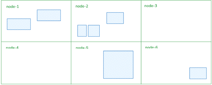
Fig 1. Within Collections, the containers of a namespace (blue) do not count as resources, themselves, but rather claim partial amounts of their underlying node resources (green)

To help further clarify the relationships between resources, domains, groups, collections, and categories, we can visualize our example.

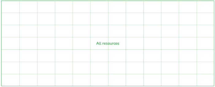
Fig 2. All resources, represented as a plane, where an (x, y) position is a single resource

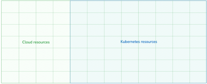
Fig 3. Resources can be divided into two domains, cloud and Kubernetes, which likely overlap

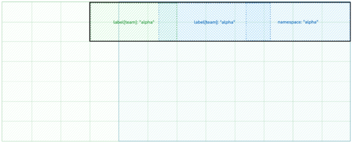
Fig 4. Groups, which might overlap, select resources using filters

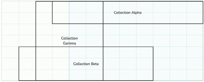
Fig 5. Collections, by virtue of their groups, contain overlapping resources from each domain

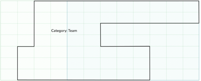
Fig 6. A category contains all the resources selected by its member collections

Now, notice a problem that might arise in our example. The same uniquely identifiable resource might appear in both the Kubernetes domain and the cloud domain. Furthermore, individual resources can be selected by more than one collection. In our example, what happens when a node that ran workloads in namespace=”alpha” also, in the cloud domain, has label[team]=”gamma”? Will Kubecost double count the costs of resources belonging to more than one group or collection?

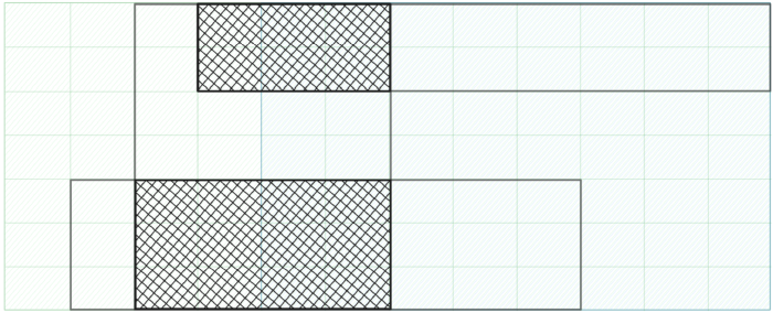
Fig 7. Resources that different groups and collections select might overlap. Here, we emphasize the resource overlap between collections at a category-level view.

As we will discuss in the next section, Kubecost resolves this problem by computing overlap, i.e., the amount of cost that is attributed to more than one group or collection by virtue of filters that select the same resource multiple times in different ways. That way, teams can assume the full cost of their resources without skewing the organization’s overall infrastructure costs.

How Does Collections Calculate Costs?

As we indicated above, there are two main ways to query collection costs:

1. Query costs for an individual collection
2. Query costs for all collections in a category

At bottom, both of these queries use the same method of querying resource costs.

Querying Resource Costs

Querying the costs associated with a selection of resources begins with two sets of filters: one for the Kubernetes domain, and one for the cloud domain. In SQL-like pseudocode, these two queries look something like the following:

-- Kubernetes query
SELECT resourceID, cost  
FROM kubernetesResources AS kr  
WHERE kr.properties MATCH kubernetesFilter  
GROUP BY resourceID  

resourceID	cost
instance-1	6.00
instance-2	4.00

-- Cloud query 
SELECT resourceID, cost 
FROM cloudResources AS cr 
WHERE cr.properties MATCH cloudFilter 

resourceID	cost
instance-2	10.00
instance-3	10.00

To get an accurate total cost of this set of resources, we’ll need to “de-duplicate” costs before aggregating them. For instance-1 we only have Kubernetes cost, and for instance-3 we only have cloud cost, so there is no de-duplication necessary. However, notice that instance-2 appears in both result sets. That is, we have the full $10.00 cloud cost of instance-2, and additionally we have $4.00 worth of Kubernetes container costs running on instance-2. To address the duplication of costs, we need to join the two queries and subtract the Kubernetes cost from the cloud cost before summing.

-- Resources query 
WITH kubernetesCosts AS ( ... ), cloudCosts AS (...), 
SELECT 
resourceID, 
kubernetesCost, 
cloudCost as fullCloudCost, 
cloudCost – kubernetesCost as finalCloudCost 
FROM kubernetesCosts AS kc 
FULL JOIN cloudCosts AS cc ON kc.resourceID = cc.resourceID 

resourceID	kubernetesCost	fullCloudCost	finalCloudCost
instance-1	6.00	0.00	0.00
instance-2	4.00	10.00	6.00
instance-3	0.00	10.00

Now we can sum our de-duplicated resource costs to get a final result.

WITH resources AS (...) 
SELECT 
SUM(kubernetesCosts) AS kubernetesCost 
SUM(finalCloudCosts) AS cloudCost 
FROM resources 

kubernetesCost	cloudCost
10.00	6.00

We can express this logic for querying resource costs as a function, which takes filters and returns costs. We will use this function to query collections and categories, below.

QueryResourceCosts(kubernetesFilters, cloudFilters) => (kubernetesCost, cloudCost) 

Querying Collection Costs

Querying collection costs largely amounts to querying the resource costs selected by both the overall collection and each group within the collection.

We will use “Collection Alpha” from the previous section as our example. Recall that this collection contains the following groups:

• Kubernetes: namespace=”alpha”
• Kubernetes: label[team]=”alpha”
• Cloud: label[team]=”alpha”

Step 1: Compute the Total Cost of the Union of All Group Filters

To compute a total cost of all resources in the collection, we only need to call our QueryResourceCosts function once, with the union of all group filters.

• kubernetesUnionFilter = (namespace="alpha") OR (label[team]="alpha")
• cloudUnionFilter = (label[team]="alpha")

The union of filters performs de-duplication for us, within a domain. Per the example, if we have Kubernetes containers that have label[team]=”alpha” and exist in namespace=”kubecost”, then they will match our filter once. If we queried for these two groups separately, we would get the same container twice.

TotalKubernetesCost, TotalCloudCost = QueryResourceCosts(kubernetesUnionFilter, cloudUnionFilter) 

Step 2: Compute the Cost of Each Group Filter Within the Collection

Although we could stop here, sometimes we want to know how much cost is attributed to each group that selects resources. Computing that calls for a very similar operation, but instead of taking the union of all filters, we will compute resource costs once per group.

KubernetesCost1, _ = QueryResourceCosts(namespace="alpha", nil) 
KubernetesCost2, _ = QueryResourceCosts(label[team]="alpha", nil) 
_, CloudCost3 = QueryResourceCosts(nil, label[team]="alpha") 

Step 3: Compute Overlap

Now we can compute an overlap figure by comparing the total cost to the sum of the group costs and subtracting the two if the latter is larger than the former.

Let’s say that in Step 1 we received:

kubernetesCost	cloudCost
60.00	200.00

And in Step 2 we received

name	kubernetesCost	cloudCost
group-1	40.00	120.00
group-2	30.00	0.00
group-3	10.00	100.00
Total	80.00	220.00

That means that our groups overlap by 300.00 - 260.00 = 40.00.

Our final result for this query would, then, look like this:

Name	Kubernetes Cost	Cloud Cost	Total Cost
Group 1	40.00	120.00	160.00
Group 2	30.00	0.00	30.00
Group 3	10.00	100.00	110.00
Overlap			-40.00
Total			260.00

Querying Category Costs

Querying category costs looks and works a lot like querying collection costs – except instead of querying for the total collection cost and the individual group costs, now we query for the total category cost and the individual collection costs.

We will use “Category Team” as our example. Recall that this category contains the following collections:

• Collection Alpha
  • Kubernetes: namespace=”alpha”
  • Kubernetes: label[team]=”alpha”
  • Cloud: label[team]=”alpha”
• Collection Beta
  • Kubernetes: label[team]=”beta”
  • Cloud: account=”123” + label[team]=”beta”
• Collection Gamma
  • Cloud: label[team]=”gamma”

Step 1: Compute the Total Cost of the Union of All Group Filters

To compute a total cost of all resources in the entire category, we need to call QueryResourceCosts with the union of all group filters in all collections.

• kubernetesUnionFilter = (namespace="alpha") OR (label[team]="alpha") OR (label[team]="beta")
• cloudUnionFilter = (label[team]="alpha") OR (account="123" + label[team]="beta") OR (label[team]="gamma")

TotalKubernetesCost, TotalCloudCost = QueryResourceCosts(kubernetesUnionFilter, cloudUnionFilter) 

Step 2: Compute the Cost of Each Group Filter Within the Collection

With categories we almost always care about how much cost each collection is contributing, so we’ll repeat “Query Collection Costs: Step 1” for each collection in the category.

k8sFilterAlpha = (namespace="alpha") OR (label[team]="alpha") 
cloudFilterAlpha = (label[team]="alpha") 
k8sCostAlpha, cloudCostAlpha = QueryResourceCosts(k8sFilterAlpha, cloudFilterAlpha) 

k8sFilterBeta = (label[team]="beta") 
cloudFilterBeta = (account="123" + label[team]="beta") 
k8sCostBeta, cloudCostBeta = QueryResourceCosts(k8sFiltersBeta, cloudFiltersBeta) 

k8sFilterGamma = nil 
cloudFilter Gamma = (label[team]="gamma") 
k8sCostGamma, cloudCostGamma = QueryResourceCosts(k8sFilterGamma, cloudFilterGamma) 

Step 3: Compute Overlap

Just as, for collections, we computed overlap by subtracting the total collection cost from the sum of the group costs, here we will compute overlap by subtracting the total category cost from the sum of the collection costs.

Let’s say that in Step 1 we received:

kubernetesCost	cloudCost
130.00	440.00

And in Step 2 we received:

name	kubernetesCost	cloudCost
Alpha	60.00	200.00
Beta	80.00	120.00
Gamma	0.00	200.00
Total	140.00	520.00

That means that our groups overlap by 680.00 - 570.00 = 110.00.

Our final result for this query would, then, look like this:

Name	Kubernetes Cost	Cloud Cost	Total Cost
Alpha	60.00	200.00	260.00
Beta	80.00	120.00	200.00
Gamma	0.00	200.00	200.00
Overlap			-110.00
Total			570.00

Querying Chargeback Costs

Querying chargeback costs for a category works a lot like querying collection costs, except instead of having a single overlap figure across the entire category, we allocate overlapping costs to collections based on their priority.

If the same resource is referenced in more than one collection within the same category, the resource will be charged to the collection with highest priority. That way, there is no “contention” over which collection owns a resource, and it is never ambiguous how to divide costs among different cost centers in an organization. However, this does require that collections in a category are arranged in a priority order, which dictates the precedence for assigning resources that might otherwise belong to multiple collections.

Allocating Idle Costs

Just as with Kubecost’s Allocations Dashboard, many users want to allocate not just the costs of their Kubernetes workloads that were used, but also the portion that remained idle, so that the full cost of Kubernetes nodes are accounted. Collections supports enabling “idle sharing” to that end.

Sharing by cluster is not recommended because that breaks the law that allows collections math to work—each resource needs to account for its own full cost, and cannot “share” its idle costs with other resources. Sharing idle by cluster means that one resource can “lend” idle cost to other resources on its cluster. We recommend, instead, sharing idle costs by node—or, in Collections language, sharing them on a per-resource basis.

Conclusion

In summary, Kubecost Collections offers teams a powerful way to measure and assign costs to multifaceted units within an organization that leverages Kubernetes as well as a suite of other cloud resources. The product and engineering teams here have worked hard to build an elegant solution to this complex problem. We hope you will install Kubecost and try it out!